..on stereometry

We try to reconstruct the image of a 3D object using images taken at different positions. Using a technique called stereometry, we will derive the depth z of the 3D object using 2D images (x,y). Consider the diagram below.





















Given that the 2 images have the same y coordinates, we could solve for z using:






where b is just the traverse distance between the 2 images and f is just the focal length of the camera. We could solve for f using the calibration technique discussed on the previous activity.

Below are the two different images of a rubik's cube taken with b=5cm.











































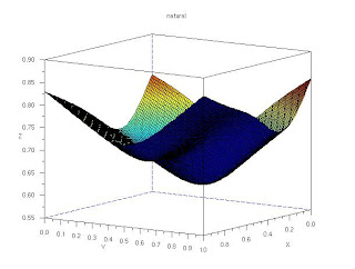
Using 25 different points (x,y), we calculated for the corresponding depth (z). Below are the 3D reconstruction using splin2d of scilab for not a knot, bilinear interpolation, natural, and monotone.
















Enlarging further, we see that the reconstructed 3D object depicts a cube. Though the resulting rendition is not a perfect cube, we were able to show the general shape of the 3D object.

















I want to give myself a 10.

..on photometric stereo

We use photometric stereo to extract the 3D shape of an object using only the information from the shadow. We estimate the shape of the object using the shading obtained from different images of different light source location.

Consider a point source of light at infinity.











The intensity I of the image is related to the vector position of the camera given by:








where N is the number of images used. We now solve for g using:




to get the normal vector n, we simply normalize it:





to derive the shape from the normals, we note that the surface elevation f(x,y) is related to the normals by:






Finally, we solve for the surface elevation using:







We apply this technique using four images of a sphere. The resulting 3D rendition is:















Indeed, the resulting shape is a sphere.

I've successfully accomplished the activity. I want to give myself a 10.

..on correcting geometric distortions

Below is an image of a "grid" capiz window. Notice that the image has a barrel distortion effect. The square grids located at the edges are much smaller than those found at the center. The center appears to be bloated while the sides are pinched. These are due to the "imperfect" lens of the camera that captured the image.

















Our goal is to correct this distortion. We use the center square grid as our reference since it is less distorted. We then determine the transformation matrix that caused the barrel effect. Let f(x,y) be the coordinates of the ideal image while g(x',y') are the coordinates of the the distorted image. To determine the transformation matrix C, we map the coordinates of the ideal image in the distorted image.










We then compute for the transformation matrix C using:






Now that we have determined the transformation matrix, we just simply copy the graylevel v(x',y') of the pixel located in g(x',y') into f(x,y). But since the calculated g(x',y') coordinates are real (pixel coordinates should be integral), we use bilinear interpolation. The graylevel of an arbitrary point is determined by the graylevel of the 4 nearest pixels encompassing that point.













We can no solve for the graylevel using:




For the remaining blank pixels in the ideal image, again we use interpolation of the four nearest corners to determine its graylevel. Below is a comparison of the original distorted image and the enhanced(ideal) image. Notice that at the lower left level, the size of the square grid for the enhanced image increased. The grid lines also become more parallel. The resulting image has lessen the effect of the distortion. The image is no more bloated.






Original distorted image











Enhanced ideal image









I think I've performed the activity successfully. The distorted image was enhanced. I want to give myself a 10.

..on camera calibration

A simple image is not an exact projection of the actual object. Some informations are lost. The task is to recover these lost details. And one of the important step is camera calibration. The goal is to know the transformation from the 3D world coordinates to the 2D image coordinates.
















Below is an image of a 3D calibration checkboard. We designated an origin and using a right-hand coordinate system, we chose 25 square corners and measured their coordinates (Yi, Zi) with respect to the origin. We also determined their real world coordinates (Xo, Yo, Zo).




















We now proceed with determining the transformation matrix a. The equation is given by














Finally, we solve for a using




To check for the accuracy, we randomly chose 4 points on the checkboard and using their real world coordinates, we calculated for their image coordinates. We measured the deviation from the theoretical value using the eucleadian distance. The results are: 1.12, 1.31, 1.44, and 0.98. These values shows that the calculated coordinates are less than 2 pixels away from the actual location. the accuracy is amazing.I was able to finish the activity with high accuracy. I want to give myself a 10.

..on preprocessing handwritten text

Below is a digitalized image of a document. Our goal is to extract the handwritten text and to remove the horizontal lines.












We remove the vertical lines using the same technique used on the previous activity(lunar image). The Fourier Transform of the image is shown below. To get rid of the horizontal lines, we have to block the frequencies corresponding to it. Thus, we introduced the filter below.
























The resulting image is free of the horizontal lines. We then binarized this image and enhanced it using morphological operations.












Below is the final image. Though we are successful in getting rid of the horizontal lines and the extraction of the handwritten text, the quality is not enhanced. The letter count is 106 which is obviously higher than the actual number of letters in the text.












I was able to finish the activity. Though the lines were successfully removed, the extracted text is not well enhanced. I hope a 9 would be reasonable.

..on binary operations

Below is an image of scattered punched paper. Our goal is approximate the size (pixel count) of a single punched paper.




















Since the image is relatively large, we cut it down into twelve 256X256 subimages. We then convert them into binary images. Below are examples of the binary images.

























These images are not ideal. We enhanced them further by applying opening and closing morphology operator. These clean the image of isolated pixel and small holes. Below are the results of the enhancement.

























We now measure the pixel count for each blob. Since the enhancement was not able to perfectly separate individual punched paper, there are big blobs on the image. We need to filter out this outliers. We do this by getting the histogram of the pixel count.


















For this particular plot, we consider only those values between 300-600 since it is in this range that we have an approximate Gaussian distribution. Finally, we take the mean of the pixel count within this range. Our result is 428.89 with a standard deviation of 71.53. To check, we processed images of individual punched paper and measured the pixel count. The average value is 456.1 with a standard deviation of 70.69. This is a 6% error.

Below is the Scilab code. I was able to implement the program such that it automatically outputs the mean pixel count and standard deviation for all images.

numt=[];
v=0;
for j=1:1:12
//upload image
dir('E:\acads\1st sem 08-09\186\activity9');
str=strcat(['C2_',string(j),'.jpg']);
image1=imread(str);

//convert to gray scale
image1=im2gray(image1);

//convert to binary
image1=im2bw(image1,229/255);
//f1=scf(1);imshow(image1);

//make structuring element
sq=ones(2,2);
se=mkfftfilter(sq,'binary',1);

//opening
C1=erode(image1,se,[1,1]);
//f2=scf(2);imshow(C1);
C2=dilate(C1,se,[1,1]);
//f3=scf(3);imshow(C2);

//closing
C3=dilate(C2,se,[1,1]);
//f4=scf(4);imshow(C3);
C4=erode(C3,se,[1,1]);
//f4=scf(2);imshow(C4);


//labeling
[mat,n]=bwlabel(C4);

//counting pixel size
val=[];
num=[];
counter=1;
for i=1:1:n
[x,y]=find(mat==i);
val(counter)=i;
num(counter)=length(x);
counter=counter+1;
end

for i=1:1:n
//mm=v+i
numt(v+i)=num(i);
end
v=v+n;

end

//histplot([10:30:800],numt);

//neglect outlier
numf=[];
c=1;
for i=1:1:length(numt)
if numt(i)>=300 & numt(i)<=600
numf(c)=numt(i);
c=c+1;
end
end

mean(numf)
stdev(numf)

I was able complete the activity. I was also able to implement the program automatically. I think I would give myself a 10 plus the bonus (5), thus a 15.=)

..on morphological operations

Below are the results when different shapes are subjected to dilation and erosion using different structuring element (SE). Dilation results to an increased size of the original image while erosion reduces the size. The resulting shape is affected by the SE. The 1st column image are the original shapes, 2nd column are the results of dilation, and the third column are the results of erosion.

1. SE: 4x4 ones























































2. SE: 2x4 ones


























































3. SE: 4x2 ones





















































4. SE: cross 5 pixel long 1 pixel thick





















































The results are consistent with the predicted sketches. As expected, the dilated image is bigger than the original while the eroded is smaller. The resulting image is affected by the SE used.

I was able to finish the activity and my results are consistent. I want to give myself a 10.