..on neural networks

On the two previous activities, we applied pattern recognition to identify the class a given image belongs to. We have used the the minimum distance classification and the linear discriminant analysis. In this activity, we introduce another method: neural networks. Neural networks mimics the way how our brain neurons work. It classifies images by learning the rule of mapping using the training set. Below is a diagram of an artificial neural network. Xi would be the inputs and Z would be the output. The goal is to determine the values of the weights Wi such that the resulting output Z matches our desired output. To do this, we train the network using examples from the training set. After determining the values for the weights Wi, we can now classify the images from the test set.















We use the same set of images form the previous activities. We consider 10 (5 training set, 5 test set) images of leaves of each kind of two different plant: Mango and an ornamental plant (I dont know the name).






Mango Leaves














Ornamental Plant Leaves







We also enhance the images as to make the classification process easier. We used the Gray World Algorithm in white balancing our images. For each class, we divided it into two groups: the training set and the test set. We use the training set to get the characteristic features of the leaves that would easily differentiate it from the other class. In this case, we used the RGB values and the eccentricity of the shape of the leaves as our four distinguishing features. Below is a table showing the four features corresponding to each of the 10 training set. These would be our input X in the neural network.

















From this training set, we determine the desired weights Wi of the network. We now classify the remaining images in the test set. The output would be 0 or 1 corresponding to the two classes (1 or 2). The table below is the summary of the results.













Like the two previous methods, neural networks have successfully classified all the 10 images. The success rate is 100%.

I was able to successfully accomplish the activity. I want to give myself a 10.

Acknowledgment to Jeric for the sample code and the discussion on neural networks.

..on probabilistic qualification

Like the previous activity, our goal is to correctly classify an image to the class which it belongs. But this time, we use a different method: the linear discriminant analysis (LDA). We use the same set of images form the previous activity. We consider 10 (5 training set, 5 test set) images of leaves of each kind of three different plant: Mango, an ornamental plant (I dont know the name), and Indian tree.






Mango Leaves














Ornamental Plant Leaves












Indian Tree Leaves








We also enhance the images as to make the classification process easier. Discussed in the previous activity, we used the Gray World Algorithm in white balancing our images. For each class, we divided it into two groups: the training set and the test set. We use the training set to get the characteristic features of the leaves that would easily differentiate it from the other class. In this case, we used the RGB values and the eccentricity of the shape of the leaves as our four distinguishing features. Below is a table showing the four features corresponding to each of the 15 training set. This would be our matrix x.



















We further group this matrix into their corresponding class: x1, x2, and x3.
x1:








x2:








x3:








We take the mean (u1, u2, u3) for each of these three matrix as well as the mean (u) of the entire matrix x. We then create the mean corrected (x1', x2',x3') matrix given by: xi'=xi-u for i=1,2,3.

We now compute for the covariance matrix given by: Ci=(xi'*xi)/ni for i=1,2,3 where ni is just the total number of trial images for class i. We further compute for the covariance matrix of the entire data given by:





where r and s corresponds for each row r and column s entry and n is just the total number of trial images. Finally, we compute for the linear discriminant function f for each class i. pi is ni/n.




The highest fi corresponds to the class where the image belongs. We do this for the 15 remaining images in the test set. The table below is the summary of the results.














Like the previous method, we have successfully classify all the 15 images. The success rate is 100%.

I was able to successfully accomplish the activity. I want to give myself a 10.

..on pattern recognition

Given an image, our goal is to correctly determine which class it belongs. Specifically, we consider 10 images of leaves of each kind of three different plant: Mango, an ornamental plant (I dont know the name), and Indian tree.






Mango Leaves














Ornamental Plant Leaves












Indian Tree Leaves









We first enhance the images as to make the classification process easier. Discussed in the previous activity, we used the Gray World Algorithm in white balancing our images.


















































For each class, we divided it into two groups: the training set and the test set. We use the training set to get the characteristic features of the leaves that would easily differentiate it from the other class. In this case, we used the RGB values and the eccentricity of the shape of the leaves as our distinguishing features. This would be our feature vector x. We take the mean m of our feature vector for the entire training set. This is given by:





where j is the class index and N is the number of samples in our training set for each class . Below is the table for the mean values for each class.





To classify which class images belongs to, we use the minimum distance classification. Taking the feature vector x of an unknown image, we determine which class mean m it is nearest to. This is given by:



where




The smallest D corresponds to the class where the unknown image belongs. We do this for the 15 remaining images in the test set. The table below is the summary of the results.














We have successfully classify all the 15 test images. The success rate is 100%.

I was able to successfully accomplish the activity. I want to give myself a 10.

Acknowledgment to Rica for uploading the images.

..on basic video processing

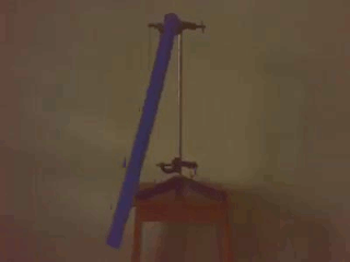
Our goal is to determine to moment of inertia (MOI) of a physical pendulum using only a video of its motion. We apply image processing techniques to extract necessary information needed to solve for the MOI. We used a flat metal ruler (mass=.0478kg, height=.635m, width=.03m) as the physical pendulum. Below is a sample video of its motion.














The MOI of a physical pendulum is given by:

I=mg(h/2)(T/2π)^2.
(source: http://cnx.org/content/m15585/latest/)

To solve for I, we have to determine the period of oscillation from the video. First, we convert the video into frames of images. In processing the images, we first apply the color image segmentation such that we pick out the moving physical pendulum away from the background. This technique has already been discussed from the previous activity. Below are the results.














Notice that the quality of the images are poor and distorted. We enhance the quality of the images using another technique previously discussed: morphological operations. We first binarized the images then apply dilation and erosion to enhance the shape of the physical pendulum.














Now that the images are enhanced, we determine the period T of the oscillation. Since the images are binarized, we could keep track of the motion of the pendulum by noting the x and y coordinates of the white pixels corresponding to the pendulum. We use the mean x and the mean y coordinate to approximate the motion of the center of mass. Below is the plot of the X axis coordinate as a function of time.














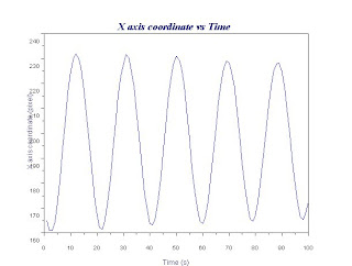
As the oscillation reaches a maximum, there would be a change in the directions of the coordinates of the center of mass. This periodic change in direction is the sinusoidal function we see in the plot above. Noting this and counting the number of frames between consecutive changes, we determine the number of frames corresponding to half the period. Since the frame rate of the video is 14.5 fps, the time interval per frame is 1/14.5=.069s. Thus the half period of the oscillation is just the number of frames times .069s.

From the processed images, the number of frames corresponding to half a period are: 10, 10, 9, 10, 9, 10, 9, 10, 10, 9. The mean value is: 9.6 frames corresponding to 0.6624s half period. Thus, the period of oscillation is 1.3248s. Using the equation above, we determine the MOI to be 6.612E-3.

To check, we determine to moment of inertia using another equation given as:

I=(m/2)(h)^2 + (m/12)(h)^2
(source: http://en.wikipedia.org/wiki/List_of_moments_of_inertia)

Noting the value of the mass=.0478kg, height=.635m, and width=.03m, the theoretical MOI is 6.428E-3. Comparing with the experimental MOI above, this corresponds to 2.86% error. The method is successful in determining the MOI of a physical pendulum using only a video of its motion.

I've successfully accomplished the activity. I want to give myself a 10.

Acknowledgment to my collaborators on the physical pendulum video gathering: Cole and Jeric.

..on color image segmentation

From a given image, our goal is to pick out the region of interest (ROI). To do this, we first have to get rid of the effect of brightness on the image (shadowing), and just consider the chromaticity. We represent the color space not by the RGB but by normalized chromaticity coordinates (NCC). Per pixel, we solve for the corresponding r,g,b values given by:




Since r+g+b=1, the chromaticity can be represented using only 2 values (r & g). Below is the normalized chromaticity space (x-axis is r and y-axis is g).











We now proceed with picking out the ROI. There are two methods: the Parametric and the Non Parametric.

Parametric

In this method, we first crop a subregion in the ROI. From this patch, we take the mean and standard deviation of r and g. We then compute for the distribution probability (we assume a Gaussian) using:





We do the same for p(g). The joint probability is just the product p(r)p(g). Below are sample the results:








Original Image


















Parametric
ROI: Blue Tiles

















Parametric
ROI: Yellow Tiles










Non Parametric (Histogram Backprojection)

In this method, we take the 2D r-g histogram of the crop subregion of the ROI. We then backproject the value to the pixel location of the original image. Below are sample the results:









Original Image
















Parametric
ROI: Blue Tiles



















Parametric
ROI: Yellow Tiles









Comparing between the two method, we could observe that the Parametric method has a better result.






Original Image














Parametric













Non Parametric









I've successfully accomplished the activity. I want to give myself a 10.

..on color image processing

Below are images taken at different white balancing.







Daylight setting under flourescent light











Cloudy setting under flourescent light















Flourescent setting under daylight







We notice that the images are wrongly balanced. The background which is supposed to be white appears otherwise. The white background for the daylight setting under flourescent light appears greenish. For the second image, the background appears grayish while for the last image, the background appears bluish. In order to correct these, we apply two popular algorithms for achieving automatic white balance: the reference white algorithm and the gray world algorithm.

Reference White Algorithm (RWA)
This method utilizes a known white image and used its RGB values as the divider. For our images, we used the background as the reference white. Below are the results of the enhancement. Notice that we have improved the color of the background as well as the colorful patches.





RWA (Daylight setting under flourescent light)














RWA (Cloudy setting under flourescent light)











RWA
(Flourescent setting under daylight)








Gray World Algorithm (GWA)
This method assumes that the world is essentially gray. Thus, we just take the average of the red, green, and blue value of the captured image and use them as the divider. Below are the resulting enhanced images. Again, the colors of the resulting images are greatly enhanced.







GWA (Daylight setting under flourescent light)













GWA (Cloudy setting under flourescent light)










GWA
(Flourescent setting under daylight)









Finally, we take an image of an ensemble of leaves having the same hue (green). This image is taken in flourescent setting under daylight. Notice that the white background appears bluish. Also, the color of the dark leaves appears black.






Flourescent setting under daylight







We improve this image using the reference white algorithm and gray world algorithm. Below are the resulting images. Both methods were able to enhance the image. The background now appears white and the color of the leaves are enhanced. Between the two methods, the resulting image from the gray world algorithm is better. The background appears really white and the color of the leaves are really distinct and clear.





RWA














GWA







I was able to successfully perform the activity. I want to give myself a 10.

Acknowledgment to Jeric for the rubik's cube and Rica for uploading the images.